5 Easy Facts About How To Use Sumif Explained
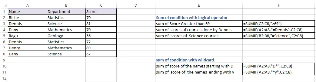
In the above screenshot, we can observe the sales of items X, Y and Z are provided. Now we require to calculate the sum of sales of X in all the three companies A, B, and also C. First, pick a cell where we want the outcomes of the sum of 'X' sales after that use feature as well as pick the array.
When the array is selected give the comma as per syntax. Later offer the "Standard" here Standard is "X" as we want to locate the AMOUNT of X product sales so provide X and also once again comma. Last, we require to choose the sum_range, right here sales is the variety which we require to add whenever the item is X for this reason select the sales variety from C 2: C 12 as revealed in the listed below screenshot.
Likewise, we can find the sales of Y and also Z likewise. See to it you are making use of the commas and a dual column for standards otherwise the formula will certainly throw an error. Normally SUMIF will certainly work on the logic AND ALSO therefore that is the factor where ever the standards match it will certainly do the addition as well as return the outcomes.
If we are using OR logic, then we can carry out AMOUNT estimation for dual criteria. For making use of OR reasoning we need to use SUMIFS as opposed to SUMIF because SUMIF can perform with solitary criteria however SUMIFS can carry out on several standards based on our requirement. Currently we will certainly take into consideration a small table which has data of sales and also revenue through online and also straight as below.
Some Ideas on Sumif Multiple Columns You Need To Know
Currently we will apply the SUMIFS formula to discover the complete sales. It is a bit various from the SUMIF as in this very first we will pick the sum range. Here sum range implies the column where the values are offered to execute enhancement or sum. Observe the above screenshot the amount is the column we need to include therefore choose the cells from C 2 to C 10 as sum_range.
Below Criteria is "Sales through direct" and "Sales with online" for this reason we need to choose the column B data from B 2 to B 10. Later we need to give the Criteria 1 and after that criteria _ range 2, criteria 2 however below we will certainly do a small change. We will certainly provide requirements 1 and standards 2 in a curly bracket like a range.
Use a filter and also filter just sales with straight and sales via online as well as choose the whole quantity as well as observe the total at the end of the display. Observe the below screenshot, I have highlighted the matter and also sum of the worths. So, the total amount should be 2274 however we got the result as 1438.
Observe the above screenshot that 1438 is the overall sales offer for sale via direct. The formula did not pick the sales with online because we provided the formula in a different format that is like a selection. Hence if we add one even more AMOUNT formula to SUMIFS after that it will certainly do the addition of both requirements.

Things about Sumif Excel
I will certainly discuss why we made use of one more AMOUNT feature and also exactly how it works. When we gave SUMIFS function with 2 requirements as in the type of an array it will compute the sum of sales through directly and also on-line separately. To obtain the sum of both we have utilized another SUM feature which will certainly add the sum of two sales.
Observe the formula we simply included the requirements X in the curly braces of a range and also it added the amount X to the existing amount quantity. In situation if you wish to make use of only SUMIF and also do not want to utilize SUMIFS after that use the formula in the below method.
In this situation initially, we provided the standards range and after that criteria 1 and also criteria 2 and also the last sum_range. In instance if we desire to execute sum based upon two columns data take into consideration the same data which we consumed to currently. We need to add another column which is called "Tax" as below.
Currently the task is to compute the amount of amount for the sales with straight and also sales with online which has "Yes" under tax obligation column. Use the formula as displayed in the listed below screenshot to get the sum of sales which has "Yes" under the Tax column. After the regular SUMIFS formula just include another requirements array which is tax column variety C 2 to C 10 as well as give requirements "Yes" in double quotes.
The Ultimate Guide To Sumif Multiple Criteria
SUMIF follows the AND logic that suggests it will certainly execute addition procedure when if requirements suits. SUMIFS will certainly follow the OR and AND reasoning that is the reason we can perform numerous requirements at once. This is an overview to SUMIF with OR in Excel. Here we review just how to make use of SUMIF with OR Criteria in Excel together with useful instances and also downloadable excel layout.
You add up multiple SUMIF features based upon OR logic, gotten each criterion separately. You require to utilize SUMIFS feature that is by default developed to sum numbers with multiple criteria, based upon AND ALSO reasoning. You can likewise make use of SUMIFS function to sum number with numerous standards, based on OR reasoning, with an array constant.
Allow's presume you have information collection of sales orders for different products, as well as you wish to sum order quantities with several requirements. If you wish to include numbers that satisfy either of the standards (OR logic) from several standards then you need to sum up 2 or more SUMIF features in a single formula.
It is vital to recognize that all of the criteria need to be satisfied on solitary or numerous arrays to summarize numbers from sum_range. The syntax of SUMIFS is; SUMIFS(sum_range, criteria_range 1, requirements 1, criteria_range 2, requirements 2, ...) Intend, you intend to sum the orders' amounts that are supplied in between two dates after that you will certainly use SUMIFS function.
sumif excel použità sumif excel with words excel sumif on filtered data